ReLL: Reproduce Learned Localization with GICP Registration of Lidar&DSM
1 Intro
This post documents my reproduction of the ICRA paper “Evaluating Global Geo-alignment for Precision Learned Autonomous Vehicle Localization using Aerial Data” (arXiv:2503.13896). I focus on implementation details that the paper omits: data preparation, dataset structure, model design, training procedure, and practical challenges I encountered and solved.
The full data pipeline and training code are open source: rongweiji/ReLL on GitHub
1.1 Outcome
Key outcomes
- Implemented the full data pipeline, including GICP registration and model training, and showed that GICP improves alignment for training.
- Compared several refinement approaches (softmax, Gaussian peak fitting). On a 0.2 m resolution dataset, the best pipeline reached translation RMS on the order of 0.1 m.
- Explored edge cases from the paper and identified a correlation between localization quality and LiDAR point “fill rate” (coverage).
1.2 Core of the paper
Brief summary of the paper
- GICP (Generalized Iterative Closest Point) is used to register LiDAR point clouds to DSM points to improve geo-alignment between modalities (paper: GICP RSS05).
- The learned localization approach trains an encoder to produce embeddings for the vehicle (LiDAR/height) and map (DSM/imagery). A cost volume (cross-correlation over a search window) measures similarity across shifts. The pipeline refines integer-pixel peaks to sub-pixel offsets using a Gaussian fit.
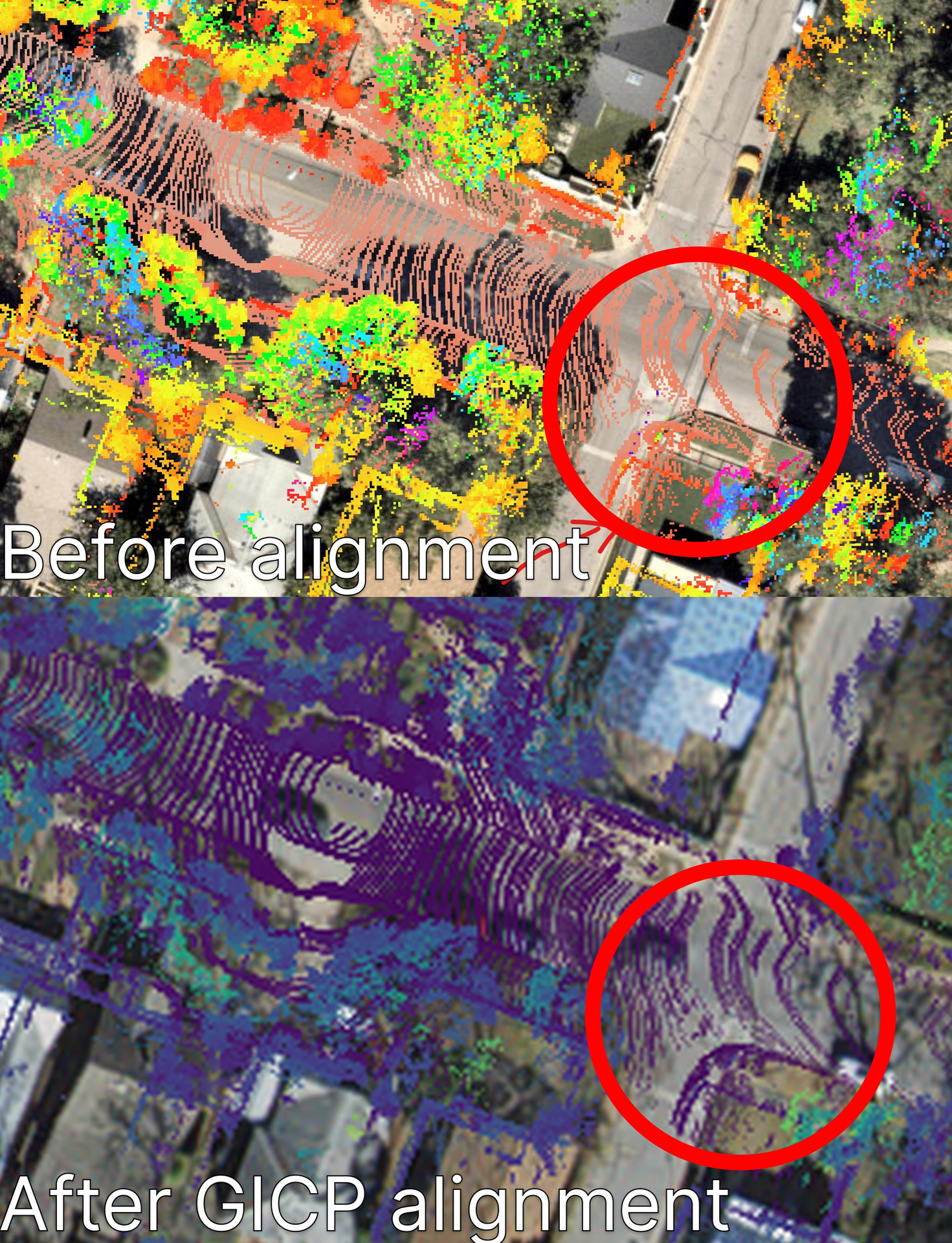 Figure 0 — Applying GICP to align LiDAR and DSM improves projection into image coordinates and helps the learned localization model.
Learned Localization: Train encoder for V&M, sliding the embeding image to measure the similartiy within a search window. Define the cost volume to measure the cross-correlation, and stack the shift to measure the shift capcity or vibrate range . using both the pixel level offset and subpixel offset by Gaussion fit to gain the presice peak.
1.3 Dataset
Dataset used
- LiDAR: Argoverse 2
- DSM: Bexar & Travis Counties Lidar (2021)
- Imagery: Capital Area Council of Governments Imagery (2022), 0.3047 m resolution
- Coordinates: UTM
- Training samples: 1,108
See the repository for dataset layout and preprocessing details: data_intro.md
2 Gaussian fit method
Gaussian fit for sub-pixel refinement
During training I use a softmax-based loss (differentiable) but apply Gaussian peak fitting only at inference to refine the correlation peak. On mixed datasets, Gaussian fitting consistently produced better refinements than naive softmax centroids.
Refinement procedure (inference)
- Extract a 3×3 patch centered on the discrete peak and clamp very small values.
- Take the log of pixel values so a Gaussian turns into a quadratic surface.
- Estimate first and second derivatives from neighbors.
- Solve for the stationary point: dx = −(d/dx) / (d2/dx2), dy = −(d/dy) / (d2/dy2).
- Clamp offsets to a safe range and add to the integer center to get a sub-pixel (x,y).
- Optionally sample the score via bilinear interpolation at the refined location.
Summary results
| Method | RMS Errors (m) | P50 (Median) (m) | P99 (99th Percentile) (m) | Mean Distance (m) | Max Distance (m) |
|---|---|---|---|---|---|
| Softmax Refinement | X: 0.2273 Y: 0.2637 Dist: 0.3481 |
X: 0.0711 Y: 0.1161 Dist: 0.1753 |
X: 1.0376 Y: 1.0816 Dist: 1.2508 |
0.2498 | 1.6772 |
| Gaussian Peak Refinement | X: 0.1907 Y: 0.2222 Dist: 0.2928 |
X: 0.0690 Y: 0.1154 Dist: 0.1701 |
X: 0.9560 Y: 1.0050 Dist: 1.2029 |
0.2090 | 1.6772 |
In short, Gaussian peak fitting converged better on my data. Because the Gaussian refinement is not differentiable in the same form, I used it only at inference rather than in the training loss.
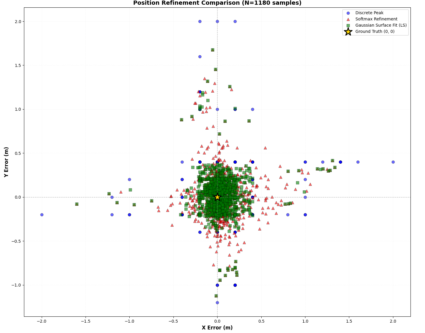 Figure 1 — Comparison of three peak-refinement methods on the mixed dataset.
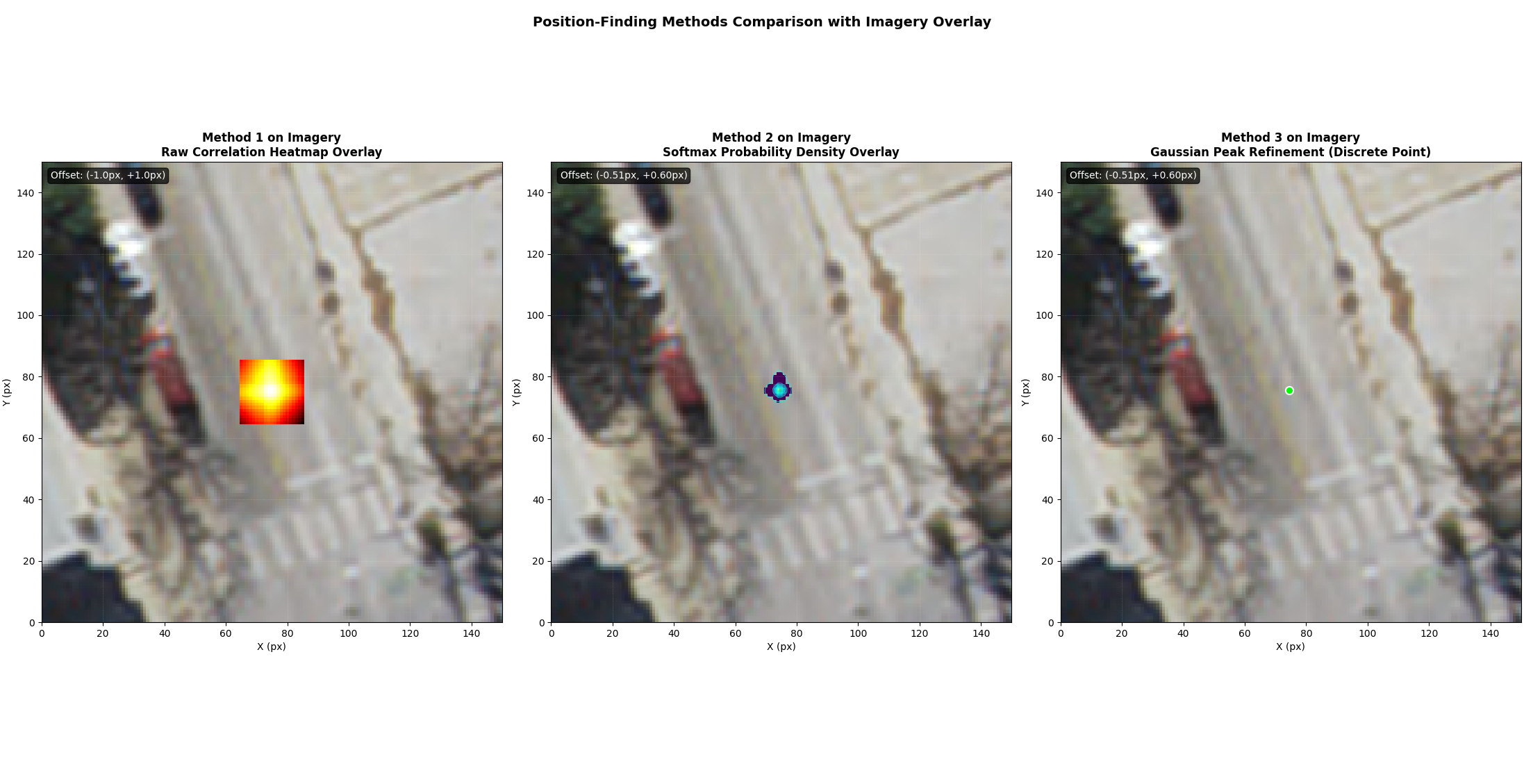 Figure 2 — Many cases show Gaussian fitting produces results comparable to softmax centroids.
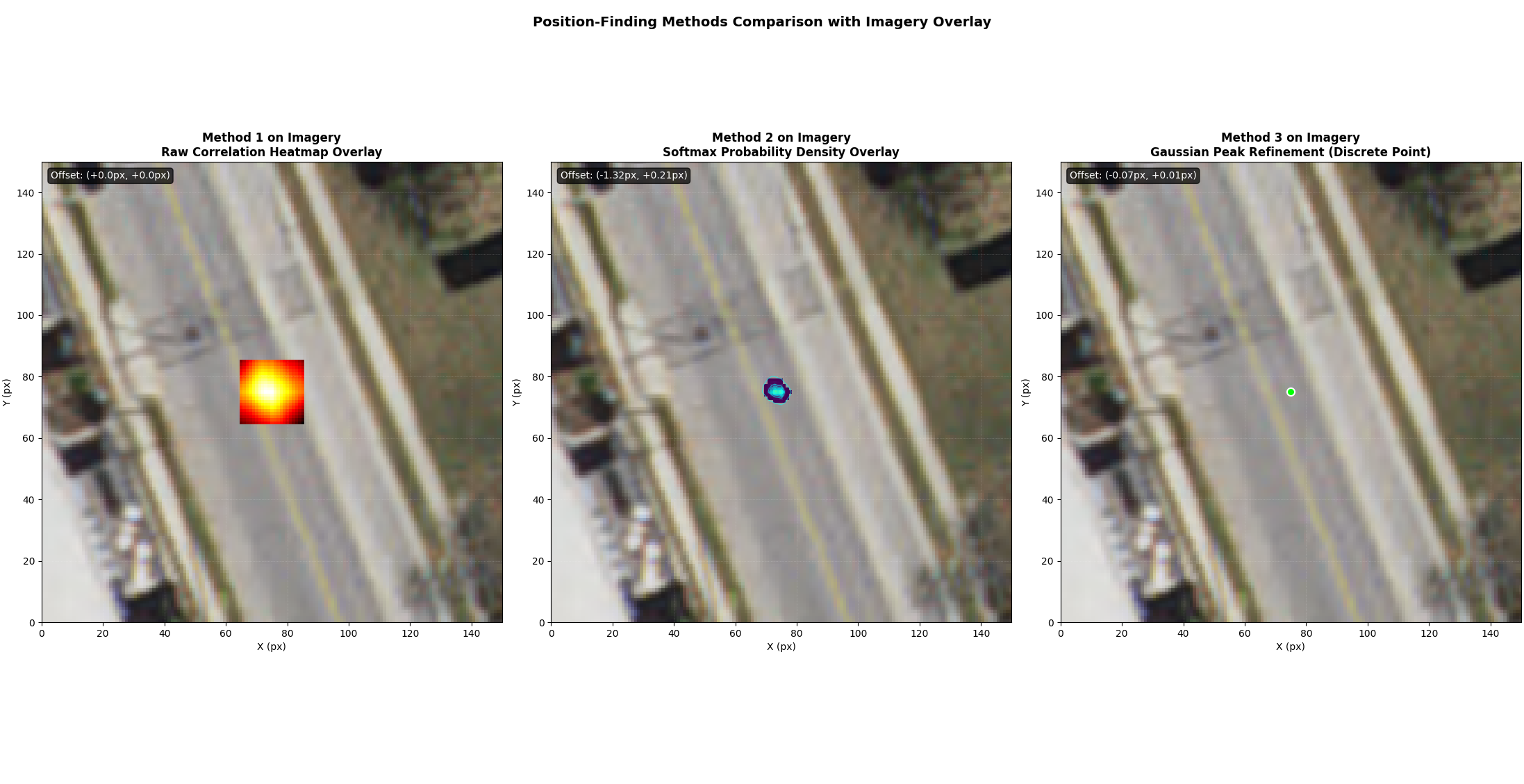 Figure 3 — Some cases where Gaussian fitting yields noticeably better results.
3 Fillment rate
LiDAR point coverage (“fill rate”)
The paper notes that localization degrades in scenes such as passing under an underpass; this matches my observations. I found localization quality correlates with LiDAR point coverage of the raster area. In scenes with poor coverage (for my example on the bridge), fewer geometric features exist, and cross-correlation peaks are less reliable.
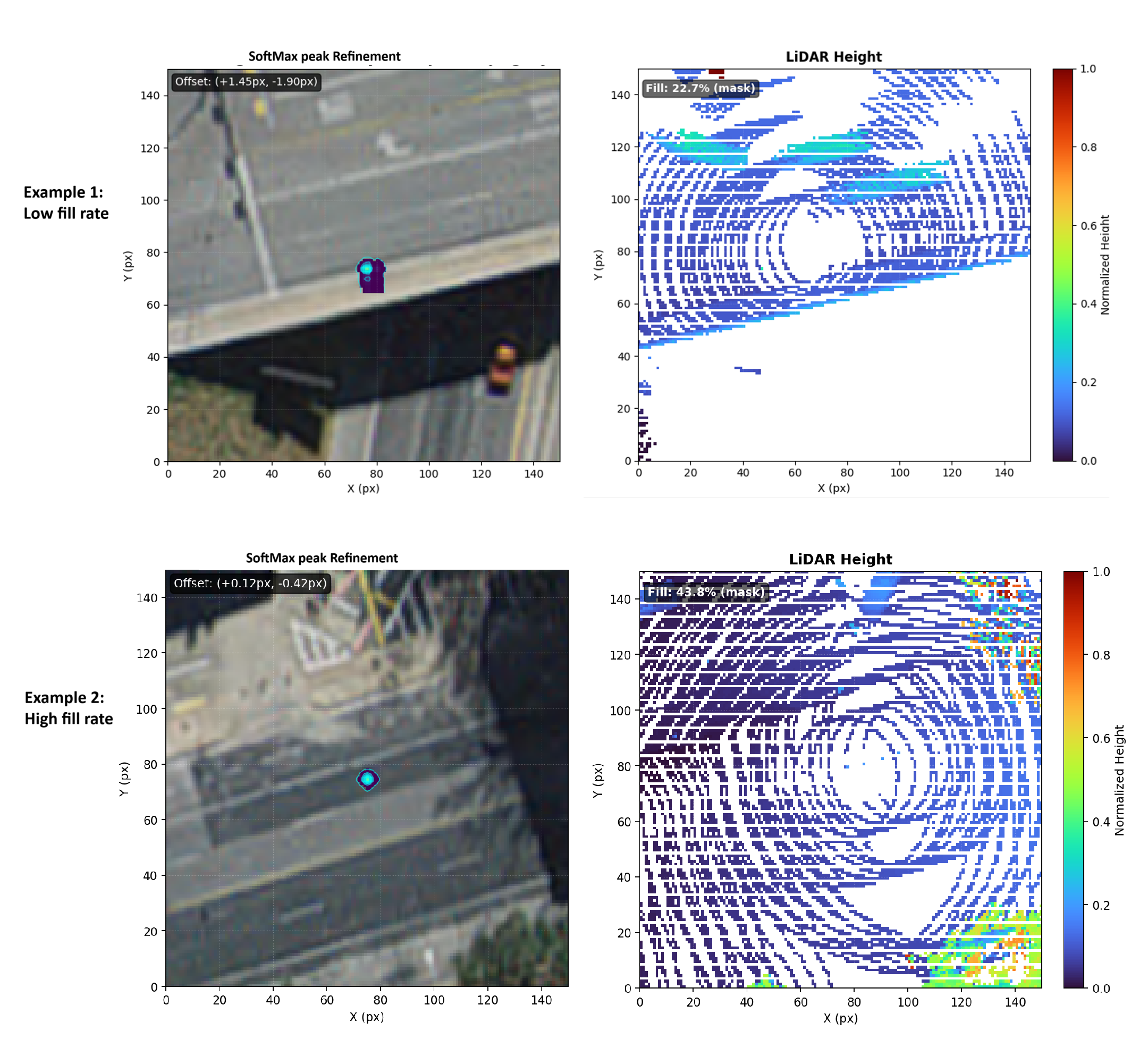 Figure 4 — Example: on bridge scene where the LiDAR point cloud does not fully cover the raster tile. Coverage correlates with poorer offsets and weaker cross-correlation peaks.
This observation explains the difference between larger-area rasters (100 × 100 m at 0.3047 m resolution) and smaller-area rasters (30 × 30 m at 0.2 m resolution). The larger raster with the coarser resolution had worse metrics; the smaller, higher-resolution tiles aligned better with the paper’s reported performance.
| Scale | Resolution (m) | Raster Size | Range (m) | x_rms (m, UTM) | y_rms (m, UTM) | θ (deg) |
|---|---|---|---|---|---|---|
| Scale 1 | 0.3047 | 329 × 329 | 100 × 100 | 0.483 | 0.423 | 0.7083 |
| Scale 2 | 0.2 | 150 × 150 | 30 × 30 | 0.105 | 0.106 | 0.3980 |
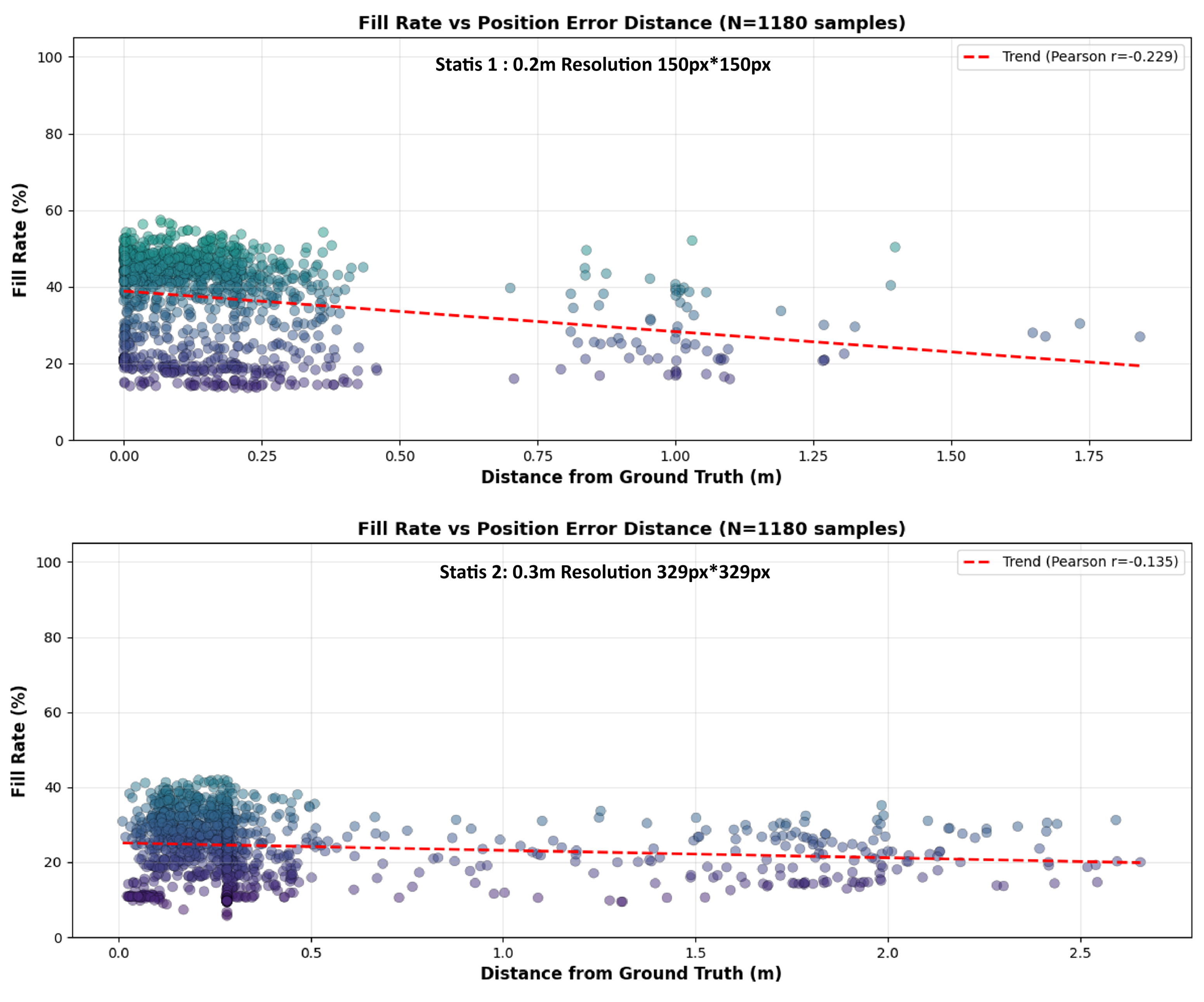 Figure 5 — Lower fill rates at bigger ranges make it harder for the model to represent geometry robustly.
4 Challenges
Major challenges and solutions
1) GICP registration and modality mismatch
When registering LiDAR to DSM, modality differences can cause local misalignments (DSM may have denser or different coverage). Filtering improved results: I keep only DSM points whose XY distance to any LiDAR point is within 0.5 m. This reduces spurious matches and yields better training alignment from GNSS-aligned data.
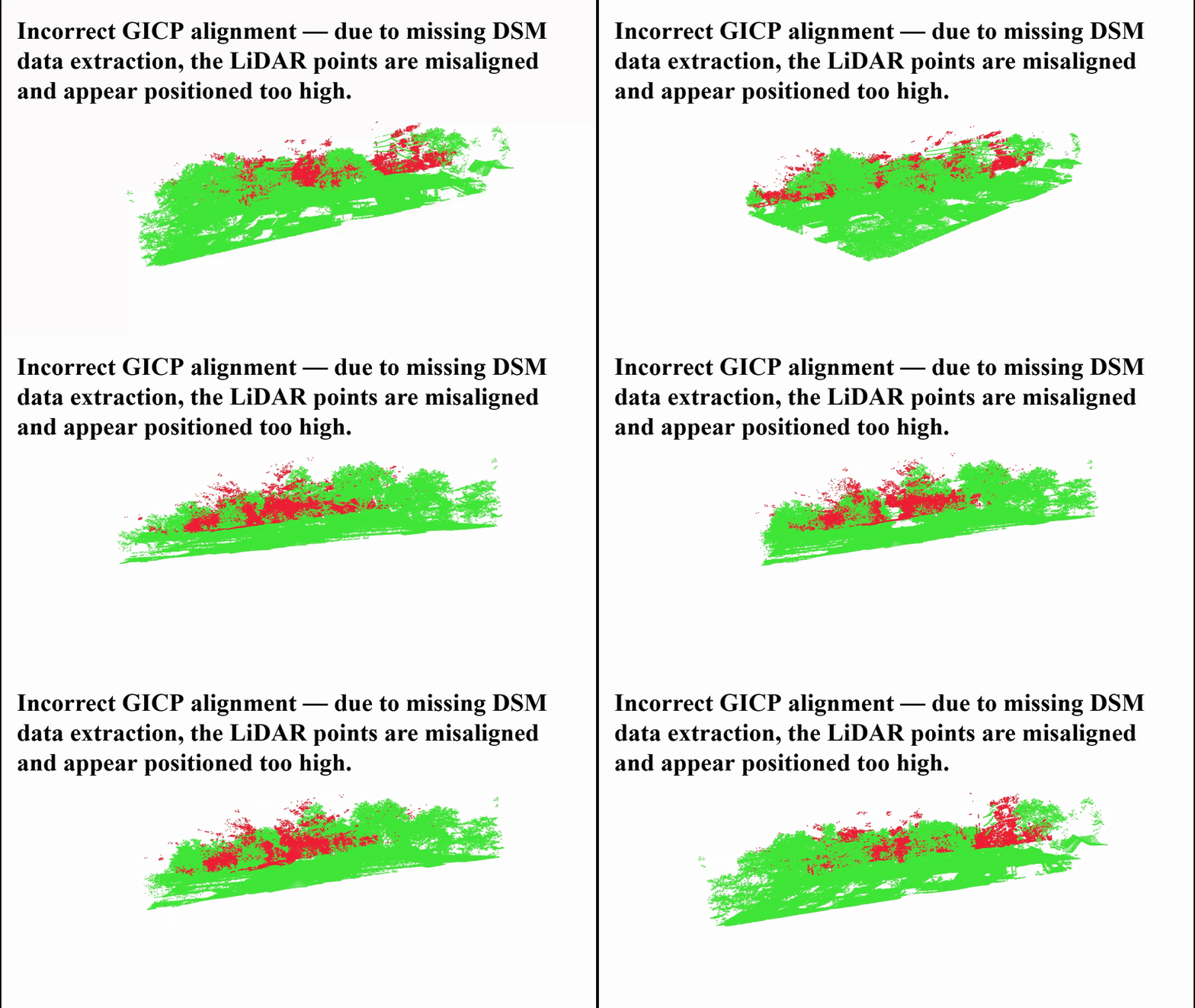 Figure 6 — Example of incorrect LiDAR–DSM alignment before filtering.
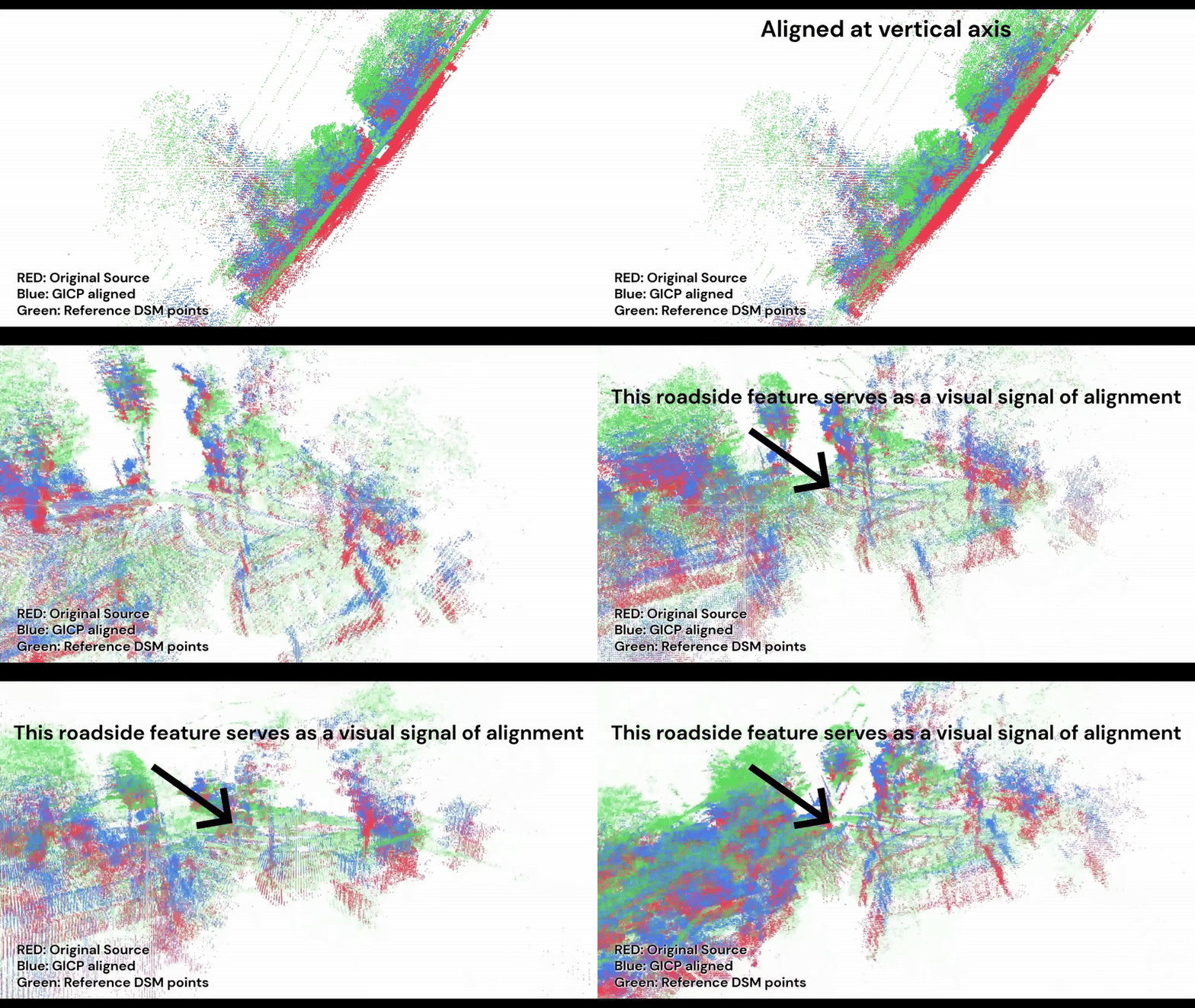 Figure 7 — Correct alignment after filtering and GICP.
2) Height normalization when rasterizing
When projecting LiDAR/DSM heights into 2D rasters, absolute altitude variation (e.g., UTM heights around 140+ m) can drown out local height features. I subtract a robust baseline (the 0.5th percentile of heights in the tile) from the raster to preserve local height contrast.
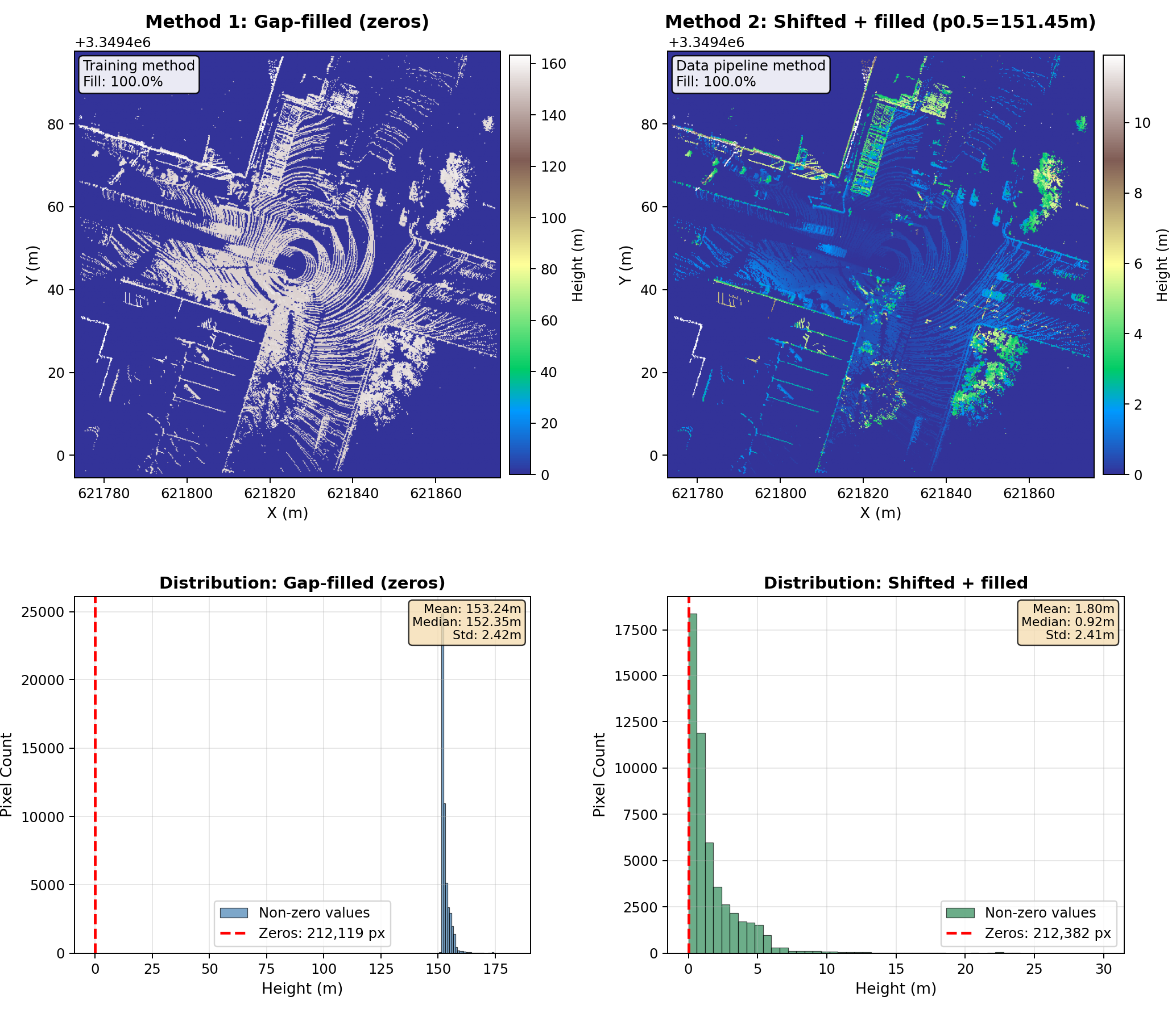 Figure 8 — Without baseline shift, the height range (0–150+) attenuates local height signals; shifting restores useful contrast.
5 Results, limitations
- Rotation (theta) convergence was weaker in my experiments than in the original paper. I tried multiple remedies but did not fully close the gap.
- Embedding visualizations show geometric patterns, but they reveal weaker height signals than the paper’s examples. That suggests the encoder architecture or preprocessing could be adjusted to emphasize height features more strongly. In my current runs I use a 4-projection dimensional output from the encoder for cross-correlation. More height signal in the embedding image indicates better performance based on limited observations.
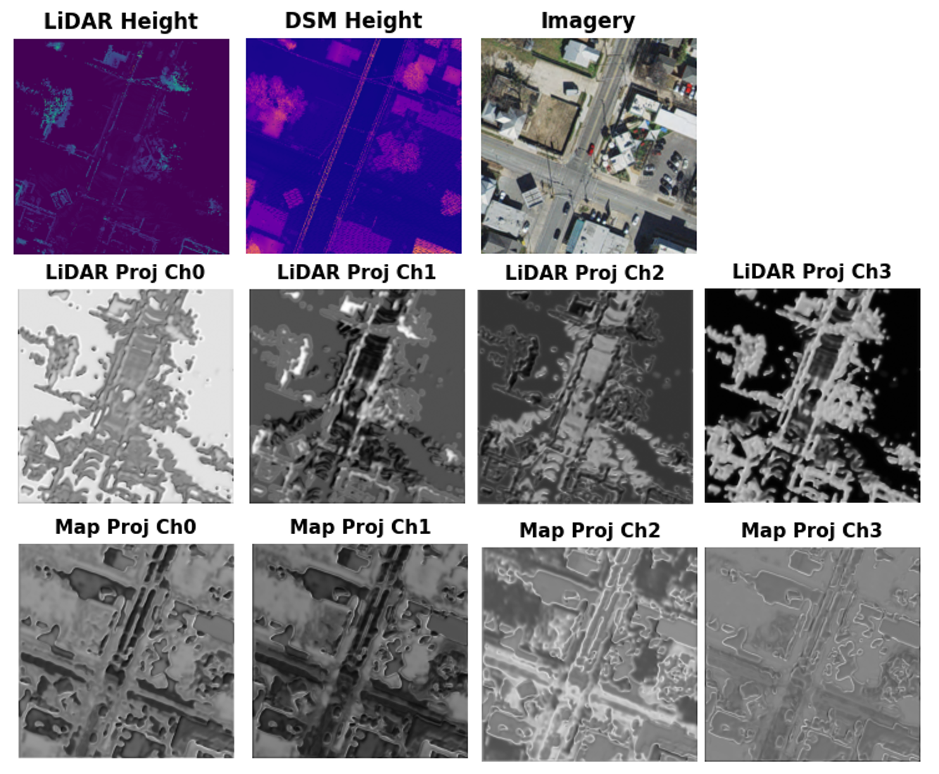 Figure 9 — Embedding visualization (example).
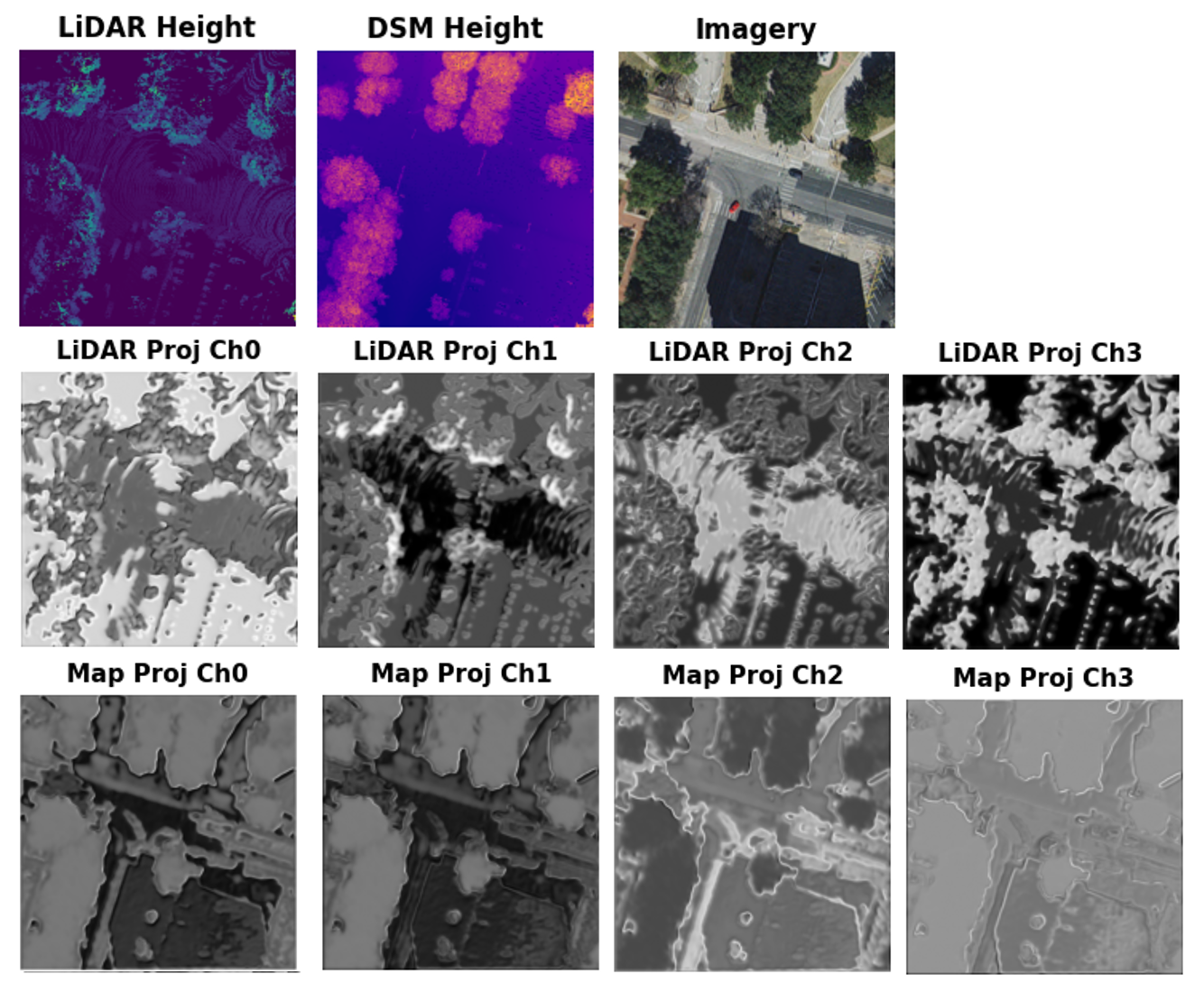 Figure 10 — Embedding visualization (example).
6 Conclusion
This reproduction confirms that careful preprocessing (GICP with filtering, height normalization) and sub-pixel refinement improve learned localization with LiDAR and DSM. Fill rate (LiDAR coverage) is important for reliable localization. The code is available at rongweiji/ReLL on GitHub if you want to reproduce or extend these experiments.